Assignment 3
Probabilistic Models of
Human and Machine Intelligence
CSCI 5822
Assigned: Tuesday 2/13/2018
Due: Thursday 2/22/2018
Goal
The goal of this assignment is to give you
more experience manipulating probabilities, performing Bayesian
inference, and exploring the Weiss et al. (2002) motion
perception model. You will also get some practice with Gaussian
distributions.
PART I
In the 2/8 lecture, I provided MATLAB code (slide 9) that implements Bayesian updating of a discrete hypothesis space for the bias of a coin (slide 8). I want you to write code (in python or whatever language you prefer) to generate my figure for the continuous distribution (slide 11) using the the Beta probability density function. In python, this function is
scipy.stats.beta.pdf.
Note that when you make plots, you will necessarily sample the
continuous density at discrete points, but your code should be
computing the parameters of the beta posterior from the
parameters of the beta prior and the observation sequence.
(I.e., don't cheat and simply make a version of the discrete
updating with many discrete levels.) Make a plot that replicates slide 11. Please include your code in the hardcopy you hand in.
PART II
In this part of the assignment, I want you to build a motion model very much like the one we discussed. I want it to handle three examples. Each example consists of two image frames on a 10x10 pixel array. The frames represent successive points in time, with red pixels for the elements that are present in frame 1, green for elements present in frame 2, and yellow for elements present in both frames 1 and 2.
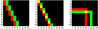
You can download python definitions for the 6 arrays from weissPatterns.py. And if you happen to be working in matlab, I also have weissPatterns.m.
Task 1
For each of these examples, compute the
(unscaled) log likelihood of motion over a range of
velocities. Assume the velocities are discrete have horizontal
and vertical components that must be one of {-2, -1, 0, 1,
2}. These velocities are expressed in pixels moved
between successive frames.
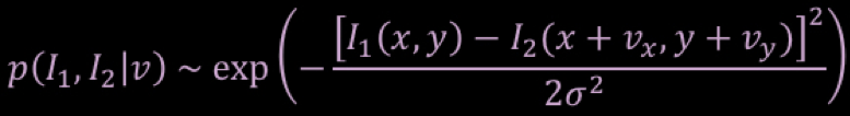
The likelihood of motion will be the product of pixelwise likelihoods for every pixel in the image. Therefore, the log likelihood of motion will be the sum of the pixelwise log likelihoods. To compute the (unscaled) log likelihood of motion for each pixel (x, y) and velocity (vx, vy), use this expression similar to that on slide 25 of the lecture notes:
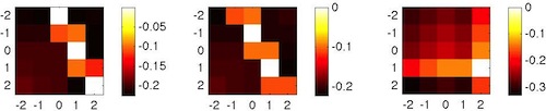
To make sure you don't go astray, here is what your result should look something like (don't worry about scaling):
The likelihood of motion will be the product of pixelwise likelihoods for every pixel in the image. Therefore, the log likelihood of motion will be the sum of the pixelwise log likelihoods. To compute the (unscaled) log likelihood of motion for each pixel (x, y) and velocity (vx, vy), use this expression similar to that on slide 25 of the lecture notes:
To make sure you don't go astray, here is what your result should look something like (don't worry about scaling):
Remember that log likelihoods are
nonpositive, and the largest possible log likelihood
value is 0. The value of σ2
will not matter for computing the (unscaled) log likelihood.
For this task, hand in your own version of a figure like the one that I made.
will not matter for computing the (unscaled) log likelihood.
For this task, hand in your own version of a figure like the one that I made.
Task 2
Now compute the (unscaled) log posterior by
incorporating the small-motion-bias prior with the free
parameter σ2/σp2=0.5.
Hand in a figure showing the (unscaled) log
posterior.
Task 3
Now compute the scaled posterior
probability over velocities. Given that there are 25 discrete
velocities, you can normalize so that the total probability of
any velocity is 1.0. Hand in a figure showing the (scaled)
posterior.
Task 4
Describe in a sentence or two how a maximum
likelihood solution (obtained using the results of Task 1)
differ from the maximum a posteriori solution (obtained from
the results of Task 2 or 3).
PART III
For part III of this assignment, you'll
implement a model from scratch has a vague relationship to the
Weiss et al. (2002) ambiguous-motion model. The model will
try to infer the direction of motion from some observations.
I'll assume that a rigid motion is being observed
involving an object that has two distictinctive visual features.
The figure below shows a snapshot of the object at two
nearby points in time. The distinctive features are the
red triangle and blue square. Let's call them R and B for
short.
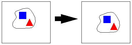
Because the features are distinctive, determining the correspondence between features at two snapshots in time is straightforward, and the velocity vector can be estimated. Assume that these measurements are noisy however, such that the x and y components of the velocity are each corrupted by independent, mean zero Gaussian noise with standard deviation σ. Thus the observation consists of four real valued numbers: Rx, Ry, Bx, and By -- respectively, the red element x and y velocities, and the blue element x and y velocities. The goal of the model is to infer the direction of motion.
To simplify, let's assume there are only four directions: up, down, left, and right. Further, the motions will all be one unit step. Thus, if the motion is to the right, then noise-free observations would be: Rx=1, Ry=0, Bx=1, By=0. If the motion is down, then the noise-free observations would be: Rx=0, Ry=-1, Bx=0, By=-1.
Formally, the model must compute P(Direction | Rx, Ry, Bx, By).
Task 1
Suppose the prior over directions is
uniform. Compute the posterior given Rx = 0.75, Ry =
-0.6, Bx = 1.4, By = -0.2. Use σ=1.
Task 2
Using the same observations, do the
computation for σ=5.
Task 3
Using the same observations, do the
computation assuming a prior in which 'down' is 5 times as
likely as 'up', 'left', or 'right'. Use σ=1.
Task 4
Using the same observations and priors, do
the computation for σ=5.