Assignment
5
Probabilistic Models of
Human and Machine Intelligence
CSCI 7222
Assigned
10/12/2013
Due 10/22/2013
Note on what to hand in
If you are confident that your code is correct and your answers are
correct, you do not need to hand in code. If you are
uncertain
about your results, then handing in code will allow me and Ron to
determine where errors were made.
Goal
The
goal of this assignment is get experience running various approximate
inference schemes using sampling, as well as to better understand Bayes
nets and continuous probability densities.
PART I
Here
is a Bayes net that relates a student's Intelligence, Major,
University, and eventual Salary.
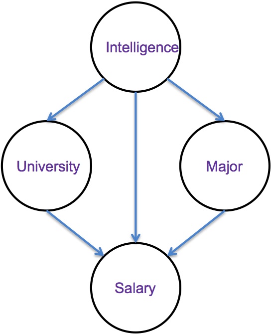
In this model, Intelligence is an individual's Intelligence Quotient (IQ), typically in the 70-130 range. University is a binary variable indicating one of two different universities that an individual attends (ucolo, metro). Major is a binary variable indicating one of two different majors that an individual might pursue (compsci, business), and Salary is the annual salary in thousands of dollars that the individual attains.
The generative model can be formulated as follows:
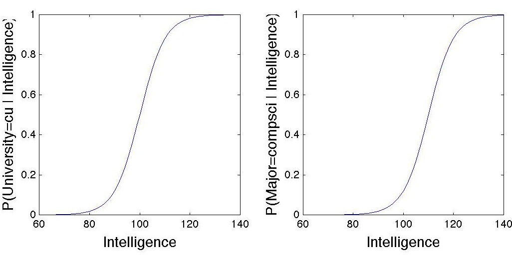
The sigmoid functions for University and Major look like this:
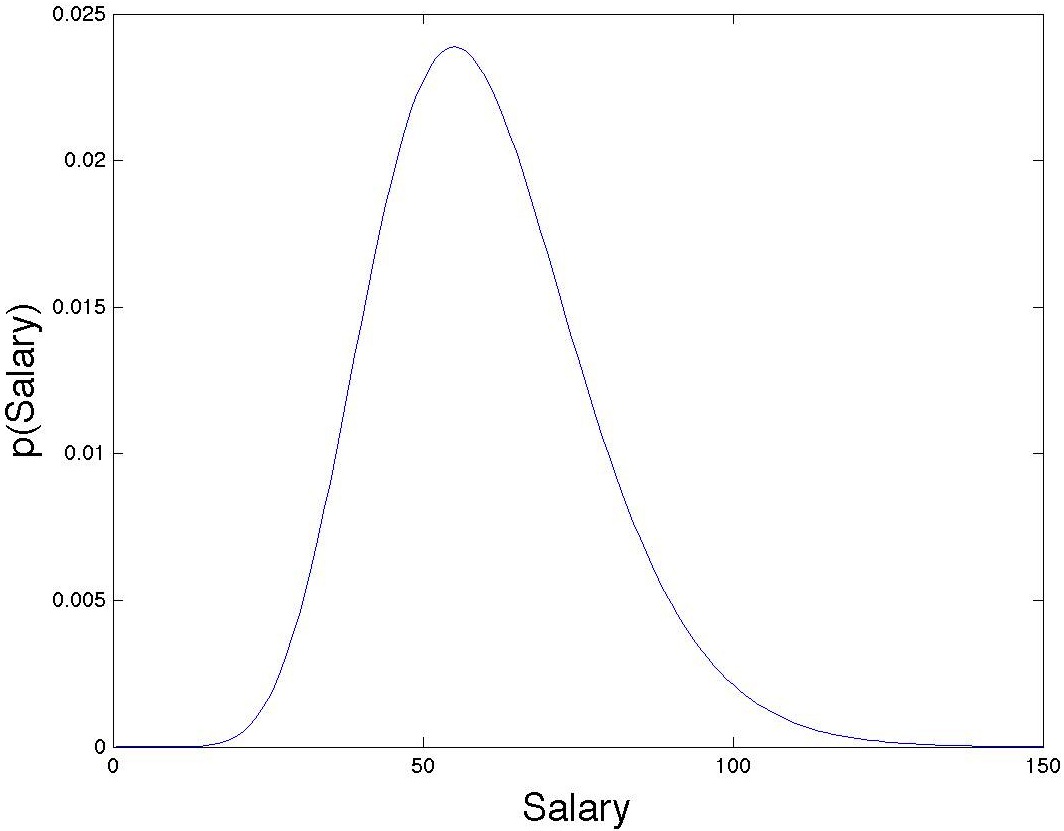
To plot a gamma density for shape=12, scale=5, use the following matlab command:
I = 100 + randn*15; % Normal(mean=100, sd=15)
M = rand < 1/(1+exp(-(I-110)/5)); % = 1 if Major=compsci, 0 if Major=business
U = rand < 1/(1+exp(-(I-100)/5)); % = 1 if University=cu, 0 if University=metro
S = gamrnd(.1 * I + M + 3 * U,5); % draw a salary from Gamma density with scale=5
For this assignment, I'd like you to estimate posterior distributions using likelihood weighted sampling (i.e., draw samples from the unconstrained graphical model that are weighted by the likelihood that Salary has the given value). Compute your estimates with at least 100,000 samples. The essential code for this computation is 8 lines in matlab, and I've given you 3 of those 8 lines!
(a) Estimate the joint posterior, P(University, Major | Salary = 120)
(b) Extimate the joint posterior, P(University, Major | Salary = 60)
(c) Estimate the joint posterior, P(University, Major | Salary = 20)
(d) I observed an interesting phenomenon in the results: The posterior probability of an individual being a CompSci major at Metro is low for each of the above conditions. What explanation can you provide for this?
In this model, Intelligence is an individual's Intelligence Quotient (IQ), typically in the 70-130 range. University is a binary variable indicating one of two different universities that an individual attends (ucolo, metro). Major is a binary variable indicating one of two different majors that an individual might pursue (compsci, business), and Salary is the annual salary in thousands of dollars that the individual attains.
The generative model can be formulated as follows:
Intelligence
~ Gaussian(mean=100, SD=15)
P(University=ucolo | Intelligence) = 1/(1+exp(-(Intelligence-100)/5))
P(University=metro | Intelligence) = 1 - P(University=ucolo | Intelligence)
P(University=ucolo | Intelligence) = 1/(1+exp(-(Intelligence-100)/5))
P(University=metro | Intelligence) = 1 - P(University=ucolo | Intelligence)
P(Major=compsci
| Intelligence) = 1/(1 + exp(-(Intelligence-110)/5))
P(Major=business | Intelligence) = 1 - P(Major=compsci | Intelligence)
P(Major=business | Intelligence) = 1 - P(Major=compsci | Intelligence)
Salary
~ Gamma(0.1 * Intelligence + (Major==compsci) + 3 *
(University==ucolo), 5)
The sigmoid functions for University and Major look like this:
To plot a gamma density for shape=12, scale=5, use the following matlab command:
plot(0:150,gampdf(0:150,12,5))
And to make sure you understand the generative model, here is matlab
code that will draw a sample from the joint distribution:I = 100 + randn*15; % Normal(mean=100, sd=15)
M = rand < 1/(1+exp(-(I-110)/5)); % = 1 if Major=compsci, 0 if Major=business
U = rand < 1/(1+exp(-(I-100)/5)); % = 1 if University=cu, 0 if University=metro
S = gamrnd(.1 * I + M + 3 * U,5); % draw a salary from Gamma density with scale=5
For this assignment, I'd like you to estimate posterior distributions using likelihood weighted sampling (i.e., draw samples from the unconstrained graphical model that are weighted by the likelihood that Salary has the given value). Compute your estimates with at least 100,000 samples. The essential code for this computation is 8 lines in matlab, and I've given you 3 of those 8 lines!
(a) Estimate the joint posterior, P(University, Major | Salary = 120)
(b) Extimate the joint posterior, P(University, Major | Salary = 60)
(c) Estimate the joint posterior, P(University, Major | Salary = 20)
(d) I observed an interesting phenomenon in the results: The posterior probability of an individual being a CompSci major at Metro is low for each of the above conditions. What explanation can you provide for this?
PART II
Suppose
x
is a 2D multivariate Gaussian
random variable, i.e., x
∼ N (μ,
Σ), where μ
= (1, 0) and Σ = (1, −0.5; −0.5, 2).
Implement Gibbs sampling to estimate the 1D marginals, p(x1) and p(x2). Plot these estimated marginals as histograms. Superimpose a plot of the exact marginals. In order to do Gibbs sampling, you will need the two conditionals, p(x1 | x2) and p(x2 | x1). Barber presents the conditional and marginal distributions of a multivariate normal distribution in 8.4.18 and 8.4.19. Wikipedia gives an alternative expression of these distributions. You may use the built-in MATLAB function to sample from a 1D Gaussian, namely randn, but you may not sample from a 2D Gaussian directly.
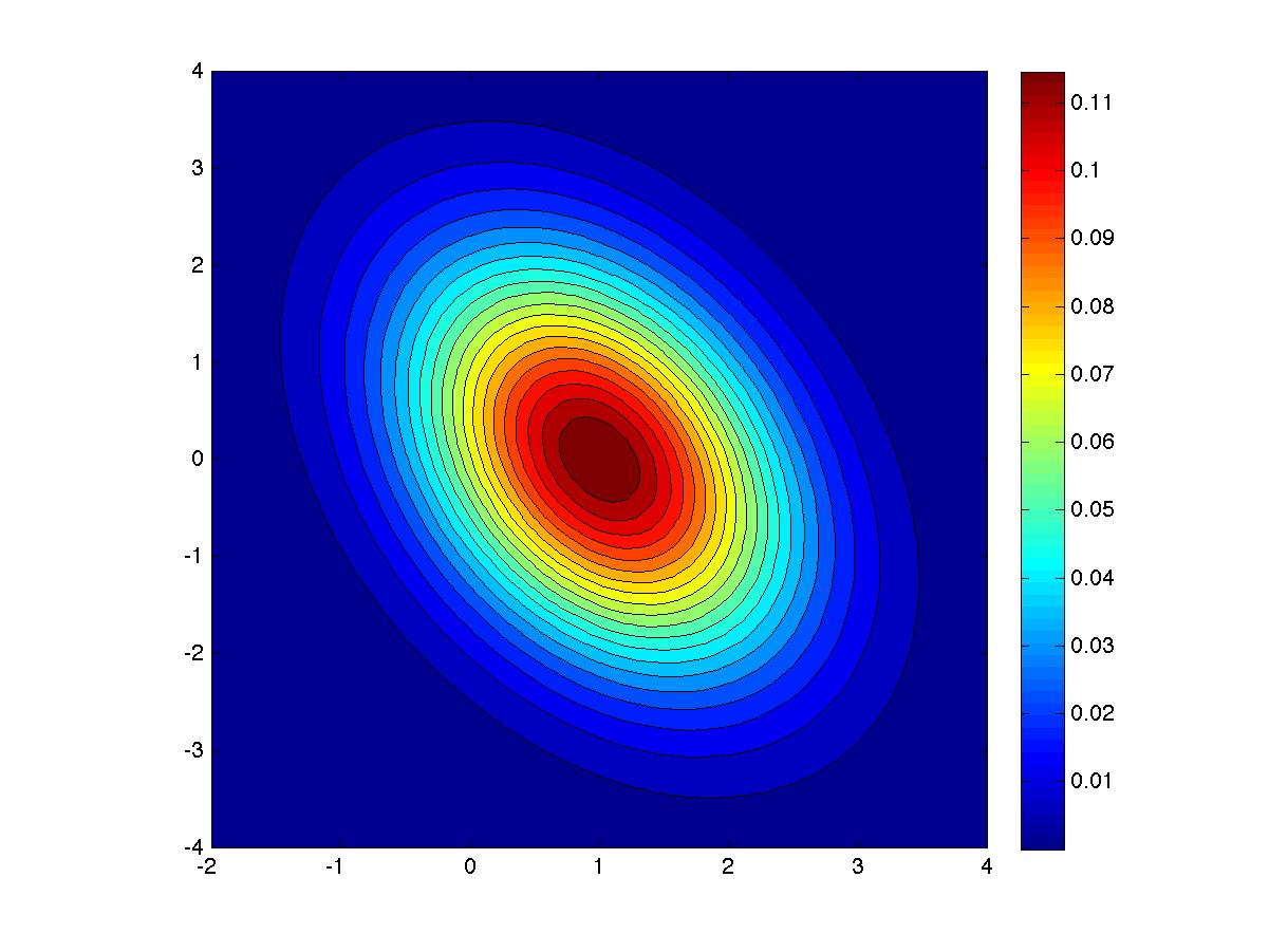
Here's what my solution looked like on a typical run.
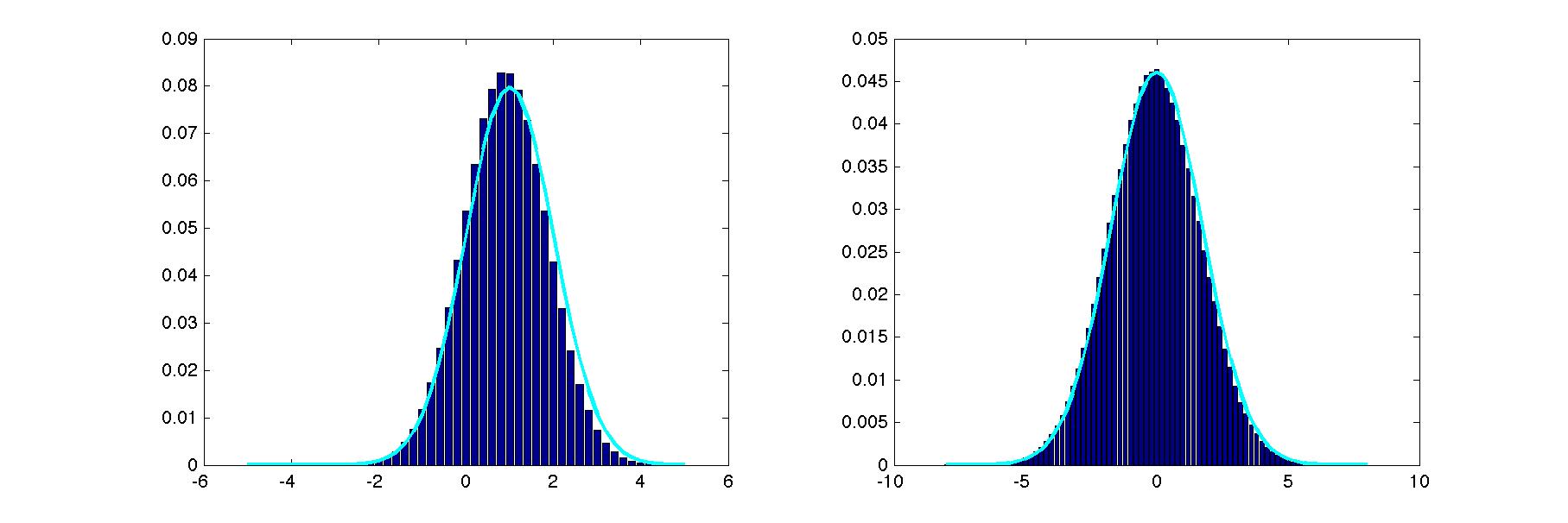
This run involved a single chain. If you see that the estimates bounce around from run to run, you may wish to run multiple chains (restarts) and combine samples, rather than one long chain. In addition to the graph showing your results, report (1) the initialization you chose, (2) the burn-in duration, (3) the number of samples obtained from each chain, (4) the number of chains (restarts) you used.
Implement Gibbs sampling to estimate the 1D marginals, p(x1) and p(x2). Plot these estimated marginals as histograms. Superimpose a plot of the exact marginals. In order to do Gibbs sampling, you will need the two conditionals, p(x1 | x2) and p(x2 | x1). Barber presents the conditional and marginal distributions of a multivariate normal distribution in 8.4.18 and 8.4.19. Wikipedia gives an alternative expression of these distributions. You may use the built-in MATLAB function to sample from a 1D Gaussian, namely randn, but you may not sample from a 2D Gaussian directly.
Here's what my solution looked like on a typical run.
This run involved a single chain. If you see that the estimates bounce around from run to run, you may wish to run multiple chains (restarts) and combine samples, rather than one long chain. In addition to the graph showing your results, report (1) the initialization you chose, (2) the burn-in duration, (3) the number of samples obtained from each chain, (4) the number of chains (restarts) you used.
PART III
Suppose
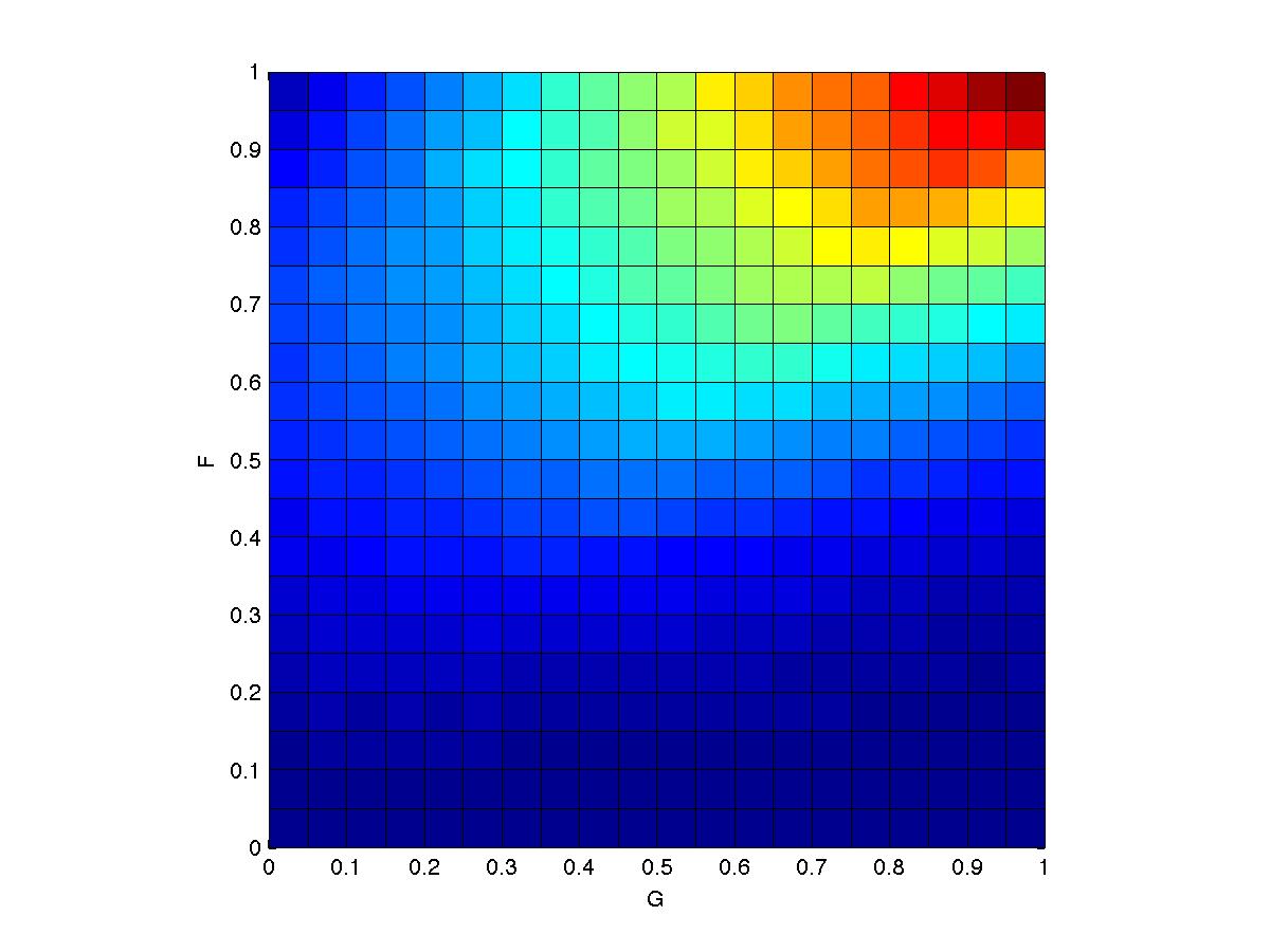
we have the following generative model for the two variables F
and G:
(a) Estimate the joint density on F and G using Metropolis-Hastings.
(b) Estimate E(FG), the expected product of F and G
(a) Estimate the joint density on F and G using Metropolis-Hastings.
(b) Estimate E(FG), the expected product of F and G
Hints
- My solution looks like this:
- I used the MATLAB stats toolbox function mhsample(). You'll discover that you really need to understand Metropolis-Hastings in order to use mhsample(), so it's not much of a shortcut. If you don't have the toolbox, Barber's text includes an M-H sampler. And if you're not using MATLAB, it's not a big deal to implement your own version of an M-H sampler.
- I decided to use a proposal distribution that is uniform, centered on the current sample with range (-s, +s). I fiddled around and picked a value of s that seemed sensible. To generate the pretty smooth distribution above, I ran with a gazillion samples.
- To plot a density for my set
of samples, smpl,
I
used the following MATLAB code:
binEdges = 0:.05:1;
N = hist3(smpl, 'Edges', {binEdges binEdges});
pcolor(binEdges, binEdges, N);
ylabel('F'); xlabel('G'); axis square - Remember that M-H sampling requires only an unnormalized probability, so you should not need to calculate ZF or ZG.
- Part (b) is one line of MATLAB code after you have obtained your set of samples.