Assignment
3
Probabilistic Models of
Human and Machine Intelligence
CSCI 7222
Assigned
9/24/2013
Due 10/1/2013
Goal
The
goal of this assignment is to give you more experience manipulating
probabilities, performing Bayesian inference, and exploring the Weiss
et al. (2002)
motion perception model. You
will also get some practice with Gaussian distributions.
PART I
In the 9/19 lecture, I provided MATLAB code (slide 7) that implements Bayesian updating of a discrete hypothesis space for the bias of a coin (slide 6). I want you to modify my code to implement the continuous hypothesis space (slide 9) using the Beta density. In matlab,
betapdf is the Beta probability
density function and betacdf is the cumulative
distribution function. Note that when you make plots, you will
necessarily sample the continuous density at discrete points. Hand in
your code as well
as your figure.
PART II
I have written MATLAB code, weissSimulation.m, which generates 3 different image examples each consisting of two image snapshots at successive points in time. The images are shown below, with red pixels being on in snapshot 1, green on in snapshot 2, and yellow on in both snapshots 1 and 2.
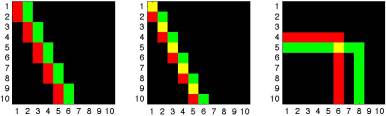
Remember that log likelihoods are nonpositive, and the largest possible log likelihood value is 0. My code uses the expression for likelihood given on slide 24 of the lecture notes on the upper half of the slide (which computes a squared difference between corresponding pixels in the two snapshots).
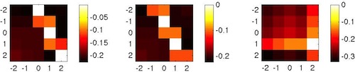
With the log likelihoods, you can select the ML (maximum likelihood) velocity. For example, in the first example, the velocity vectors (1,0), (2,2) and (0,-2) are all equally likely interpretations of the motion; for the third example, the maximum likelihood velocity vector is (2,1). For Part I of the homework, I want you to modify my code to compute the posterior distribution over likelihoods by incorporating Weiss's small-motion-bias prior with the free parameter σ2/σp2. (Remember, the free parameter is a ratio of variances; there's only one parameter value to pick.)
Hand in this posterior distribution over velocities for two values of the constant, and indicate the two values you've chosen. Try to choose constants such that the MAP solution is different for the two values. The posterior distribution over velocities should look like the likelihood ditsribution (and you can use the same matlab code), but it should incorporate the prior.
PART III
For part III of this assignment, you'll implement a model from scratch
has a
vague
relationship
to the Weiss et al. (2002) ambiguous-motion model. The model
will try to infer the direction of motion
from some observations. I'll assume that a rigid motion is
being observed involving an object that has two distictinctive visual
features. The figure below shows a snapshot of the object at
two nearby points in time. The distinctive features are the
red triangle and blue square. Let's call them R and B for
short.
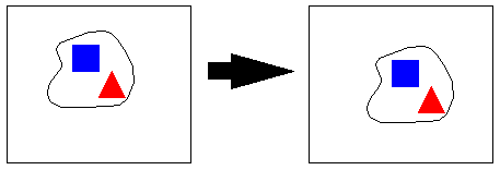
Because the features are distinctive, determining the correspondence between features at two snapshots in time is straightforward, and the velocity vector can be estimated. Assume that these measurements are noisy however, such that the x and y components of the velocity are each corrupted by independent, mean zero Gaussian noise with standard deviation σ. Thus the observation consists of four real valued numbers: Rx, Ry, Bx, and By -- respectively, the red element x and y velocities, and the blue element x and y velocities. The goal of the model is to infer the direction of motion.
To simplify, let's assume there are only four directions: up, down, left, and right. Further, the motions will all be one unit step. Thus, if the motion is to the right, then noise-free observations would be: Rx=1, Ry=0, Bx=1, By=0. If the motion is down, then the noise-free observations would be: Rx=0, Ry=-1, Bx=0, By=-1.
Formally, the model must compute P(Direction | Rx, Ry, Bx, By).
Task 1
Suppose
the prior over directions is uniform. Compute the posterior
given Rx = 0.75, Ry = -0.6, Bx = 1.4, By = -0.2. Use σ=1.
Task 2
Using
the same observations, do the computation for σ=5.
Task 3
Using
the same observations, do the computation assuming a prior in which
'down' is 5 times as likely as 'up', 'left', and 'right'.
Use σ=1.
Task 4
Using
the same observations and priors, do the computation for σ=5.
What to hand in
I
would like hardcopies
of your work. It's easier for you than putting together a
single
word / pdf document. And it's easier for me than keeping tabs
on
electronic documents. It would be good for you to hand in the
code in case there's a problem with your results.