We will present compositions of extended finite state machines.
Recall a deterministic EFSM from the previous lecture. \[(Q, X, I, O, q_0, x_0, \delta),\]
The system is deterministic (since \(\delta\) is a function). Thus for every pair \((q, x)\), with mode \(q \in Q\) and \(x \in D(X)\), and each input \(y \in D(I)\), we have exactly one next state \[ (q',x') := \delta(q,x,y)\,.\]
The model for a nondeterministic system differs in the following ways
Often it is hard to describe a monolithic system but easier to build it from parts using compositions. We will start with two basic types of compositions that can be used to build machines: parallel and sequential compositions. Note that more complex models can be built by combining many components in parallel and sequential compositions.
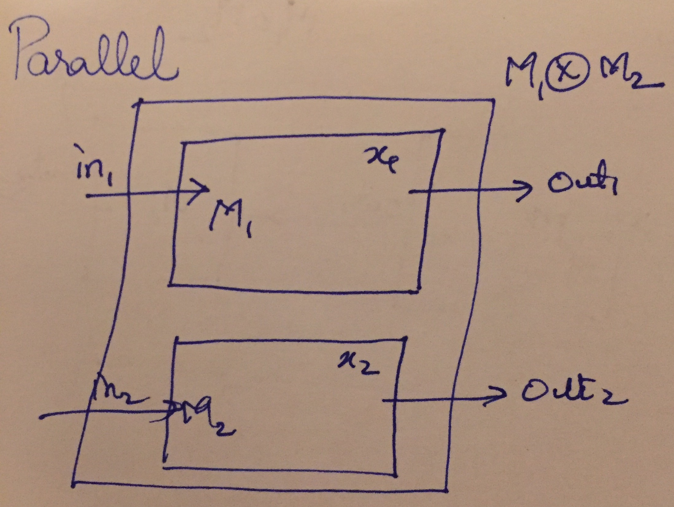
First, we illustrate the parallel composition \(M_1 \otimes M_2\) of two systems \(M_1\), \(M_2\) as shown in the figure below:
The composed system has the combined inputs of \(M_1, M_2\), combined internal states and outputs of the two individual systems.
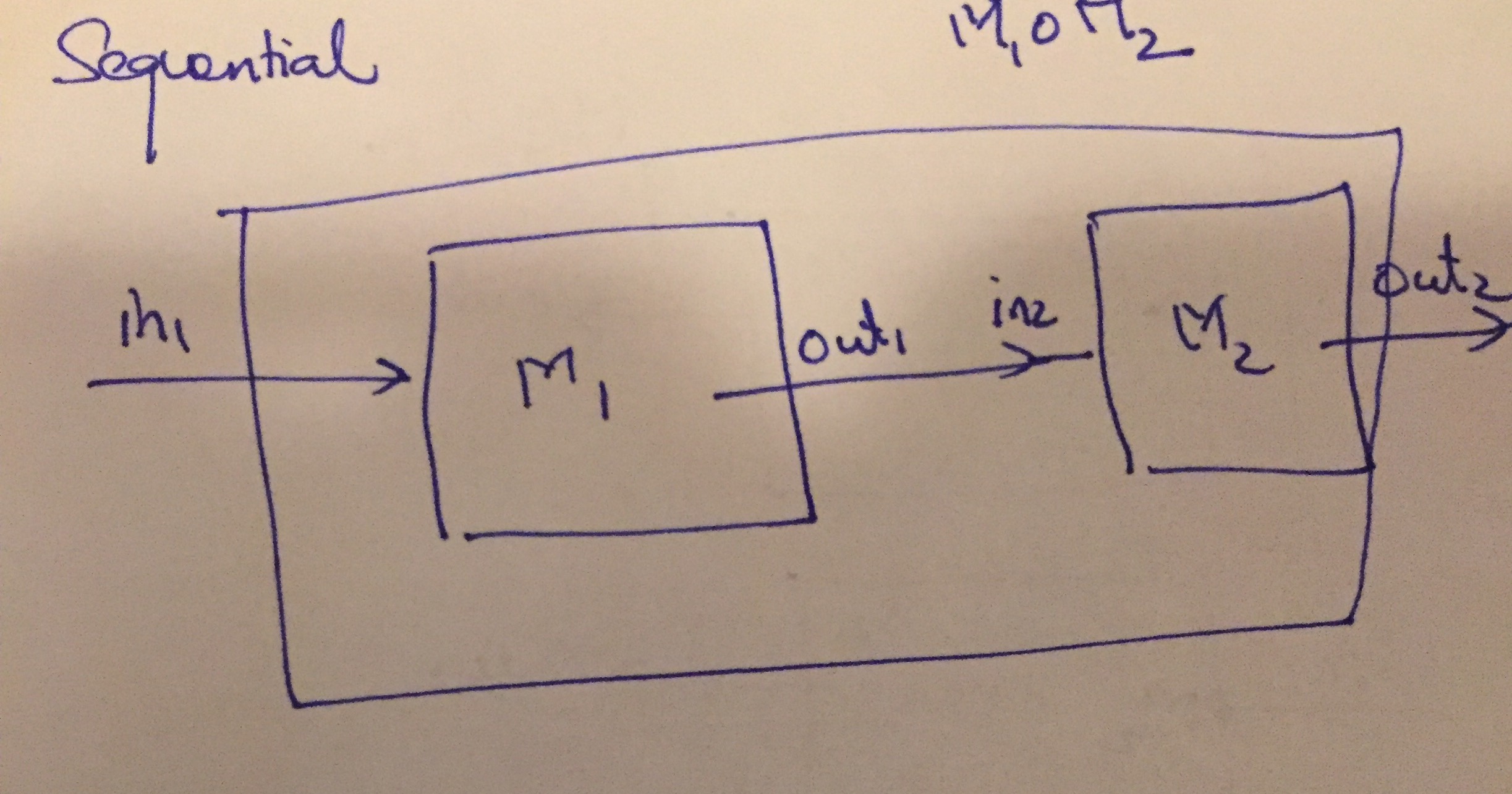
Next, we illustrate the sequential composition \(M_1 \circ M_2\) of two systems \(M_1\), \(M_2\) below:
Sequential Composition
The composed system has the input of \(M_1\) and the output of \(M_2\), but combines the internal states of \(M_1\) and \(M_2\).
For simplicity, let us define two deterministic EFSMS:
\[M_1: (Q_1, X_1, I_1, O_1, q_{0,1}, x_{0,1}, \delta_1),\ \ M_2: (Q_2, X_2, I_2, O_2, q_{0,2}, x_{0,2}, \delta_2) \,.\]
In other words, the parallel composition behaves as if both machines execute in parallel.
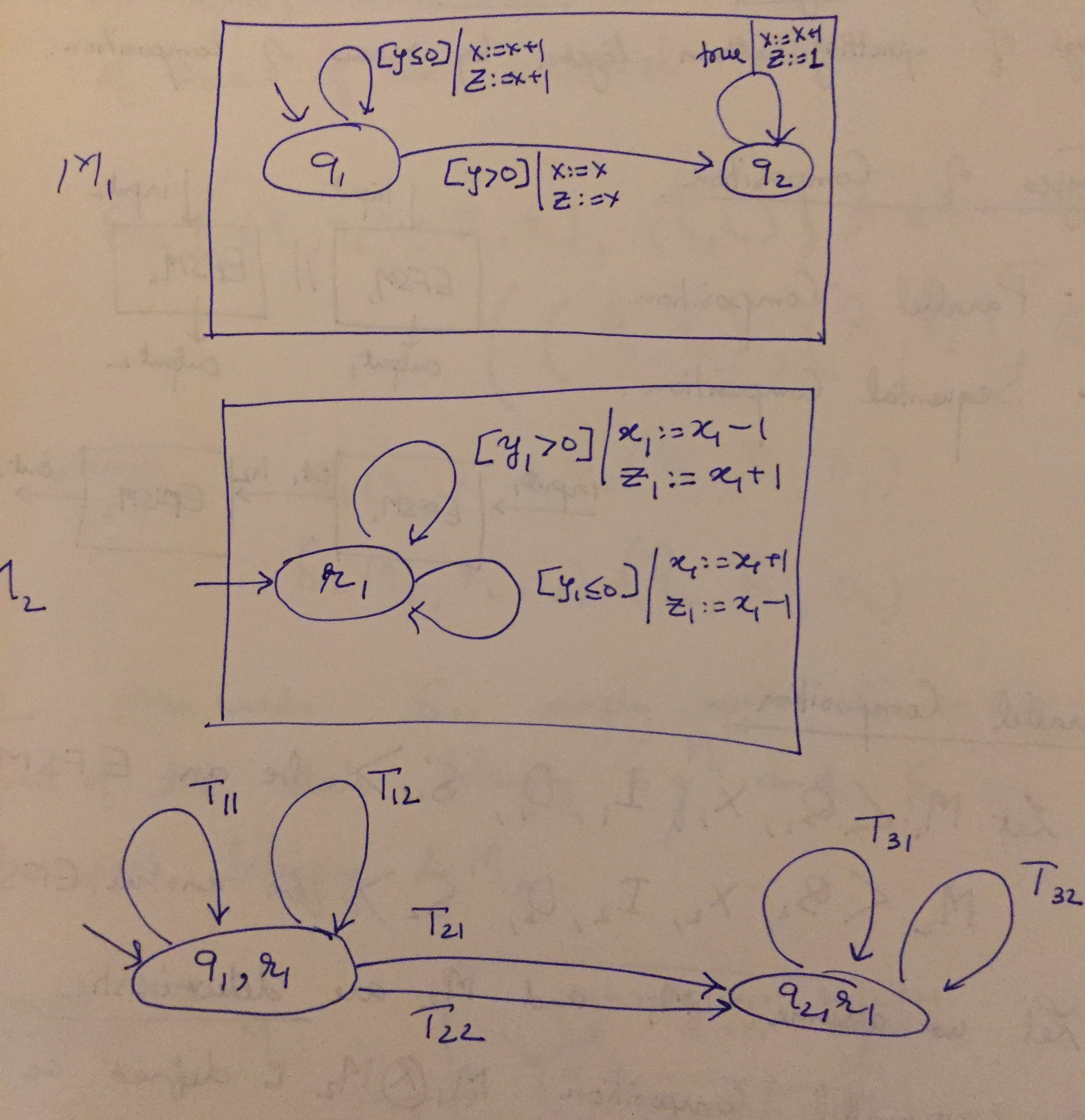
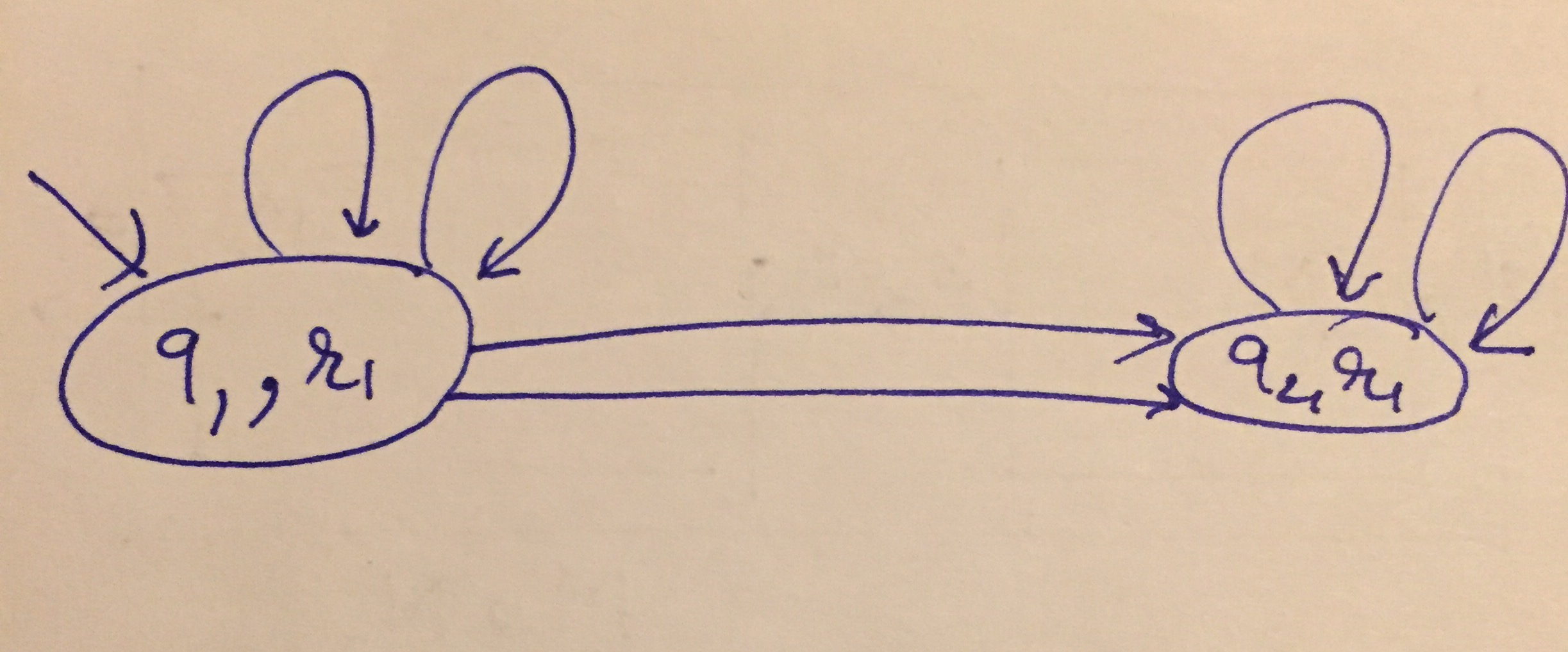
Consider two machines shown in the diagram below:
Parallel Composition Example
The parallel composition \(M_1 \otimes M_2\) has two modes \((q_1, r_1)\) and \((q_2, r_1)\) given as the product of the two state variables.
Its inputs are now \(\{y, y_1\}\), outputs are \(\{z, z_1\}\) and internal states are \(\{x, x_1\}\).
There are six transitions between them given by taking the product of each transition of \(M_1\) with that of \(M_2\). They are given by
\[\begin{array}{lll} \hline \text{Source/Dest} & Guard & Update \\ \hline (q_1,r_1) \rightarrow (q_1, r_1) & y \leq 0 \land y_1 > 0 & x := x+1, x_1 := x_1 -1, z := x+1 , z_1 := x_1 +1 \\ \hline (q_1,r_1) \rightarrow (q_1, r_1) & y \leq 0 \land y_1 \leq 0 & x := x+1, x_1 := x_1 +1, z := x+1 , z_1 := x_1 -1 \\ \hline (q_1,r_1) \rightarrow (q_2, r_1) & y > 0 \land y_1 > 0 & x := x, x_1 := x_1 -1, z := x , z_1 := x_1 +1 \\ \hline (q_1,r_1) \rightarrow (q_2, r_1) & y > 0 \land y_1 \leq 0 & x := x, x_1 := x_1 +1, z := x , z_1 := x_1 -1 \\ \hline (q_2,r_1) \rightarrow (q_2, r_1) & y_1 > 0 & x := x+1, x_1 := x_1 -1, z := 1 , z_1 := x_1 +1 \\ \hline (q_2,r_1) \rightarrow (q_2, r_1) & y_1 \leq 0 & x := x+1, x_1 := x_1 +1, z := 1, z_1 := x_1 -1 \\ \hline \end{array}\]
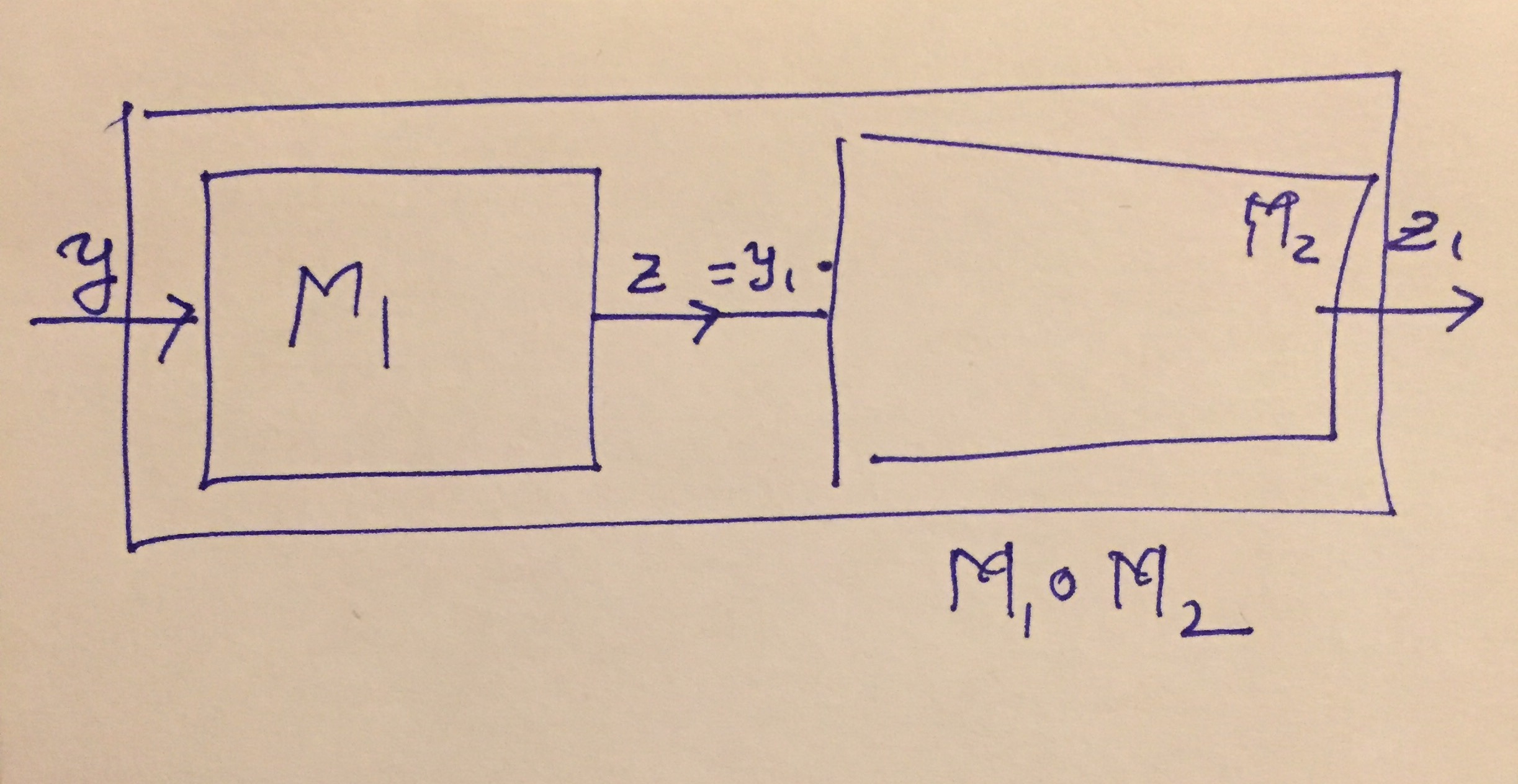
Note here that machine 1 and 2 make a move in a single cycle. First machine \(M_1\) computs an output \(z_1\) for the input \(y_1\) and current state \((q_1, x_1)\). Next, machine \(M_2\) operates on \(z_1\) as input and produces \(z_2\), the final output.
Let us revisit the parallel composition example above and instead sequentially compose the two machines \(M_1\) and \(M_2\) as defined above.
Sequential Composition Diagram
The sequential composition's structure is the same as that of the parallel composition.
Sequential Composition Structure
However, the transitions are now going to be completely different. Note that now, the input is \(y\) and output is \(z_1\). We can no longer talk about \(z\) or \(y_1\) in the composed machine since that connection is internal to the machine.
\[\begin{array}{lll} \hline \text{Source/Dest} & Guard & Update \\ \hline (q_1,r_1) \rightarrow (q_1, r_1) & y \leq 0 \land x+1 > 0 & x := x+1, x_1 := x_1 -1, z_1 := x_1 +1 \\ \hline (q_1,r_1) \rightarrow (q_1, r_1) & y \leq 0 \land x+1 \leq 0 & x := x+1, x_1 := x_1 +1, z_1 := x_1 -1 \\ \hline (q_1,r_1) \rightarrow (q_2, r_1) & y > 0 \land x > 0 & x := x, x_1 := x_1 -1, z_1 := x_1 +1 \\ \hline (q_1,r_1) \rightarrow (q_2, r_1) & y > 0 \land x \leq 0 & x := x, x_1 := x_1 +1, z_1 := x_1 -1 \\ \hline (q_2,r_1) \rightarrow (q_2, r_1) & 1 > 0 & x := x+1, x_1 := x_1 -1, z_1 := x_1 +1 \\ \hline (q_2,r_1) \rightarrow (q_2, r_1) & 1 \leq 0 & x := x+1, x_1 := x_1 +1, z_1 := x_1 -1 \\ \hline \end{array}\]
In particular, there is a simple way to derive each transition for the sequential composition from the table for the parallel one. Just apply the equality \(y_1 = z\) to substitute for \(y_1\) in terms of \(z\) and the result of \(z\) in terms of \(y,x\) every place. Then we eliminate \(z\) and \(y_1\) themselves from the transitions. Note that in particular, the last transition has the guard \(1 \leq 0\) or \(\text{false}\). It can be safely deleted since it will never be taken.
Often machines executing in parallel will need to synchronize their actions by sending or receiving events between each other. This functionality makes the description of many complex systems quite simple and succinct. At the same time, it can lead to some subtle bugs in these systems.
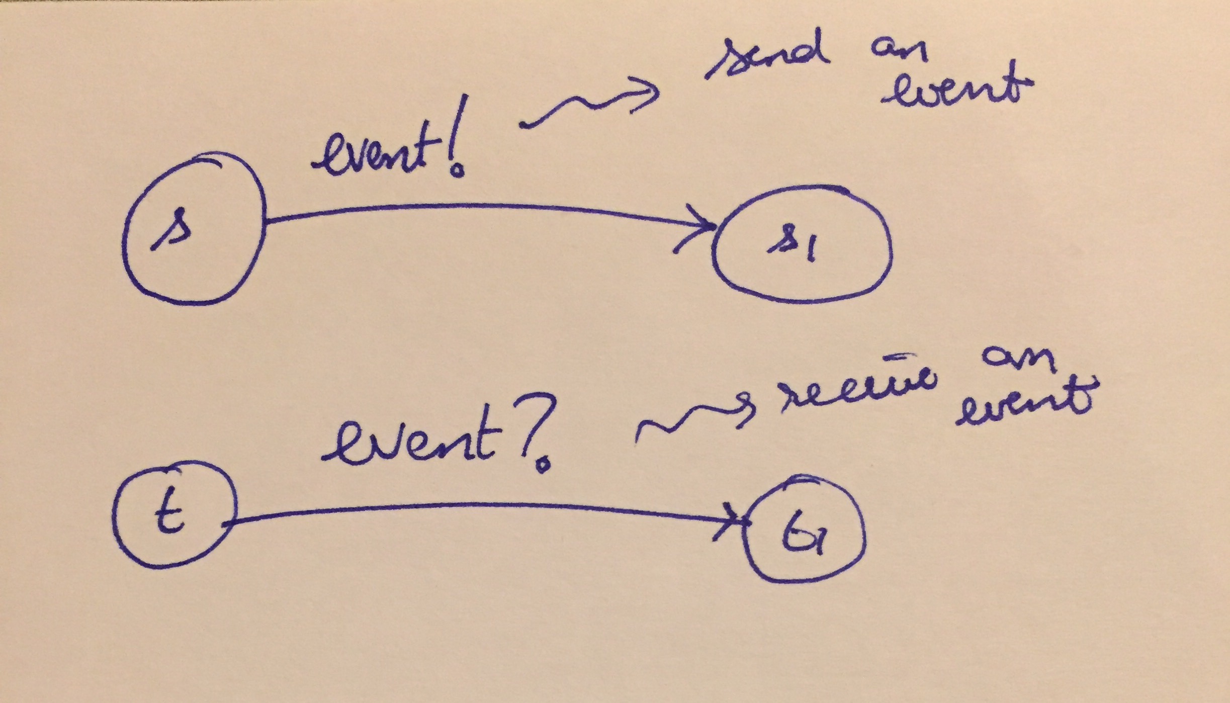
We will study just one type of synchronization for now: synchronous rendezvous that allows machines to send/receive events on transitions.
Rendezvous Communication in EFSMs
There are many possible types of communication mechanisms implemented in actual systems in practice. For example, the rendezvous construct is inspired by the ADA programming language. Likewise, Java has wait/notify statements that also have the flavor of sending and receiving events. Similarly, if you are familiar with the message passing interface (MPI) used in large scale distributed computers, the different nodes can communicate by sending and receiving messages, as well.
In EFSMs, we will have the following constraints: 1. Any time an edge \(s \rightarrow s_1\) wishes to send an event 'event!', there must be a receiver \(t \rightarrow t_1\) executed in the parallel machine at the same cycle to receive the message. In other words, we will have blocking sends. 2. Any time an edge \(t \rightarrow t_1\) has to receive a message 'event?' to execute, there must be an edge in the parallel machine that will send that event in that cycle.
Note that each send must be matched by a receive but the send/receive themselves can exchange places in the events.
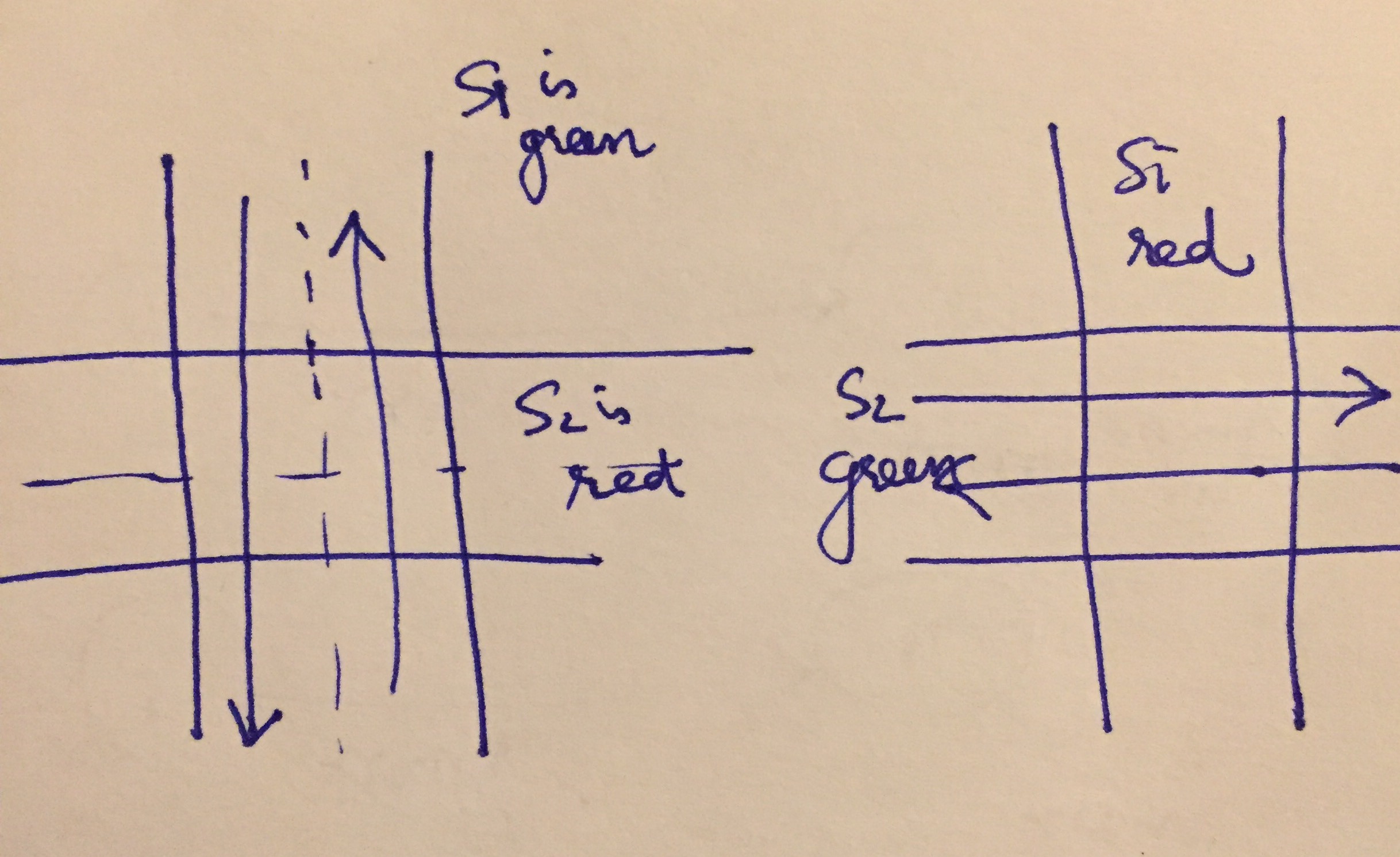
Consider two traffic lights \(S_1\) and \(S_2\) that control traffic going NS and EW on a road, respectively.
Traffic Light Example
Using message passing, we can write down two separate implementations of each traffic light that can synchronize with each other to avoid both lights simultaneously green or yellow at the same time. Likewise, we can also avoid the lights being simultaneously red.
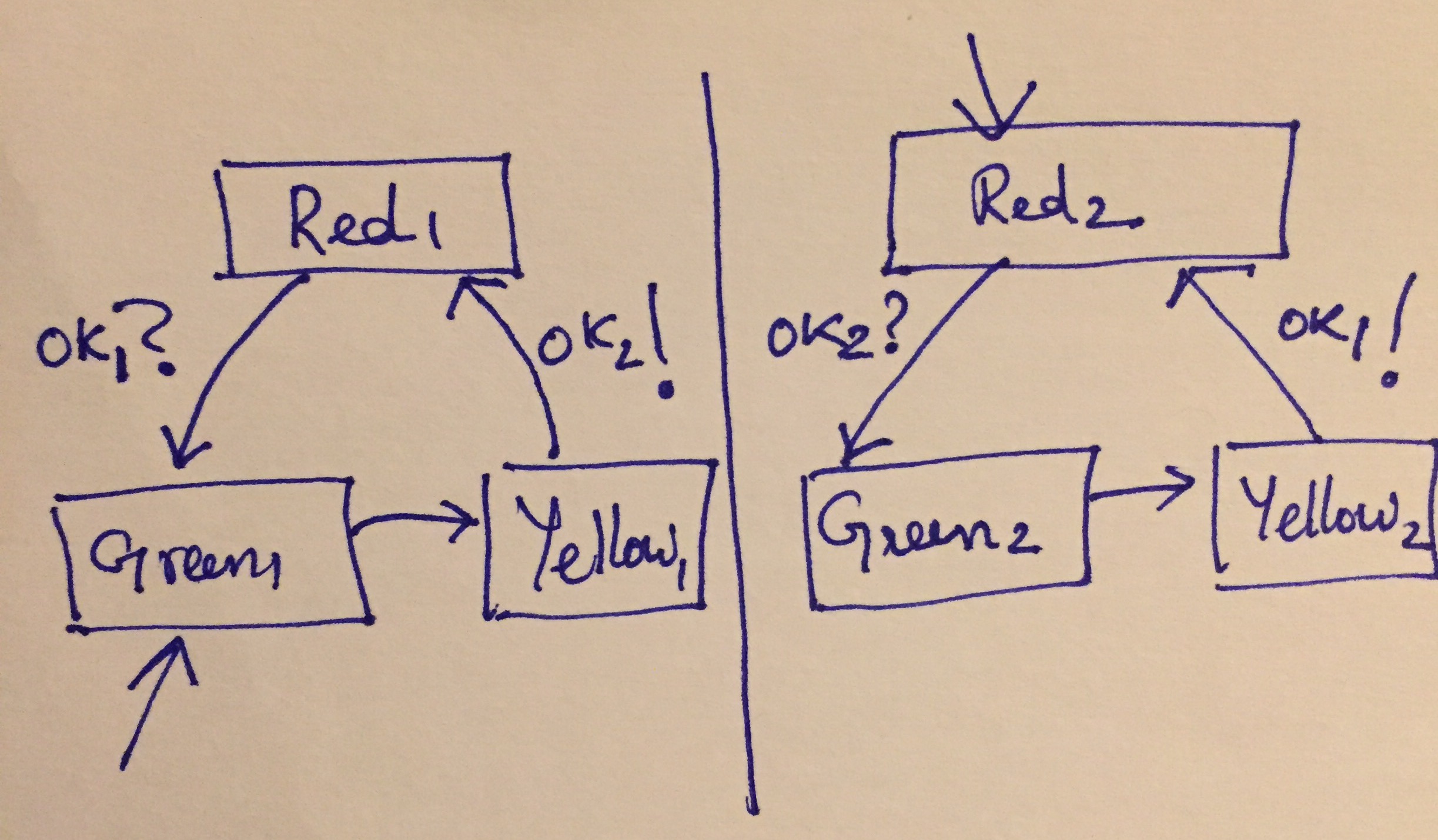
Traffic Light EFSMs
For convenience, we do not consider inputs, internal states or outputs yet. There is a self loop on each red/yellow node that is to be taken if the events on the transitions cannot be sent/received.
We can now extend EFSMs with events. Let \(E := \{ e_1, \ldots, e_k \}\) be a collection of events that can be sent or received along edges in an EFSM.
An EFSM extended with events has the following information along each transition:
Once the EFSM is extended with events, consider the parallel compositition of two transitions
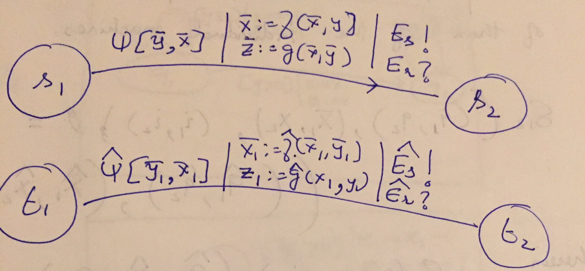
Parallel Transitions with Events
In particular, each transition is shown with a guard predicate, updates on the internal states and outputs. But additionally, we have
First transition sends events \(E_s\) and receives events \(E_r\),
Second transition sends events \(\widehat{E_s}\) and receives \(\widehat{E_r}\).
The composed transition goes from \((s_1, t_1)\) to \((s_2, t_2)\) with guard \(\Psi_1 \land \Psi_2\) and actions that simply combine the assignments to the internal states and outputs. The combined transition sends the events:
\((E_s \setminus \widehat{E_r}) \cup (\widehat{E_s} \setminus E_r)\), I.e, every event sent by each transition that is not already received by the other will remain as an event to be sent in the composed transition.
\((E_r \setminus \widehat{E_s}) \cup (\widehat{E_r} \setminus E_s)\), I.e, every event received by each transition that is not already sent by the other will remain as an event to be received when taking the composed transition.