Last revised 19 July 2016
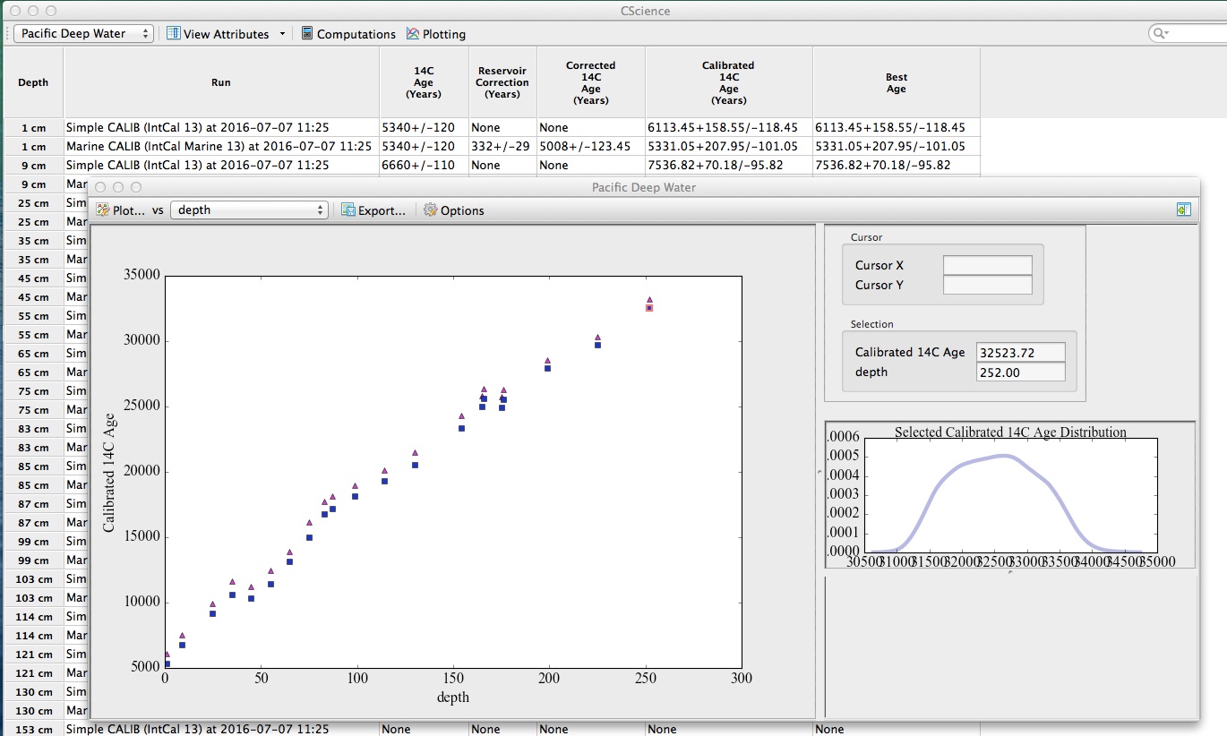
In the screenshot below, I'm using CSciBox to analyze the Pacific Deep Water core using two different analysis workflows. (An "analysis workflow" is a series of computations that act upon the data and produce results like calibrated 14C ages.) The names of the workflows that I ran on this core are shown in the "Run" column of the interface that's peeking out from behind the plot: one called "Marine CALIB (IntCal Marine 13)" that applies a reservoir age correction to the 14C ages and then calibrates the corrected ages using the IntCal 2013 calibration curve, and another called "Simple CALIB (IntCal 13)" that skips the reservoir age correction step. The "14C Age (Years)" column is the input data; other columns contain the results of the two different workflows---e.g., the corrected and/or calibrated ages at each depth in the core. (Please ignore the "Best Age" column; more on that below.)
|
Running those workflows is simple; you simply click on the "Computations" button at the top of the CSciBox window and choose the one you want to apply to the data in the workspace:
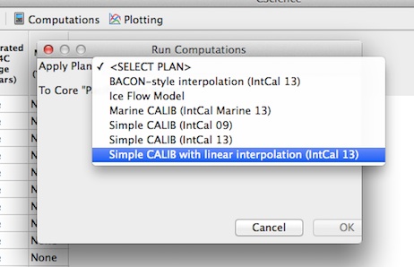 |
After you hit the "OK" button, that workflow will then run, requesting additional information, as necessary, via dialog boxes and putting its results in the appropriate columns in the grid.
On the first screenshot above, the calibrated ages with and without the reservoir age correction are shown as magenta triangles and blue squares on the plot, respectively. These icons depict the means of the distributions of the associated quantities. You can see the full distributions by clicking on a point. In the plot above, I've clicked on the oldest blue square; that's why there's a red outline around it. The lower-right panel of that screenshot shows the full distribution of calibrated 14C ages at that point that were produced by the "Simple CALIB (IntCal 13)" analysis workflow.
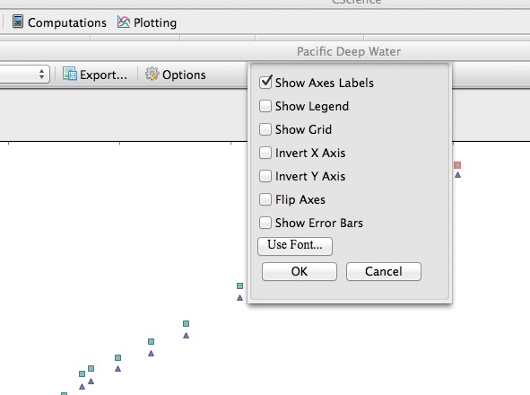
You can customize your plot further by clicking the "Options" bar in the plotting window:
 |
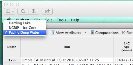
The July 2016 version of CSciBox "ships" with three cores: a section of the NGRIP ice core and two sediment cores, one marine and one lake. The second video on our "tutorials" webpage demonstrates how to import and export data records in various formats. If you want to see what records are in CSciBox's database -- and switch back and forth between which one is in your workspace -- you use the dropdown at the top left (the one that shows the name of the core that's in your workspace):
 |
 |
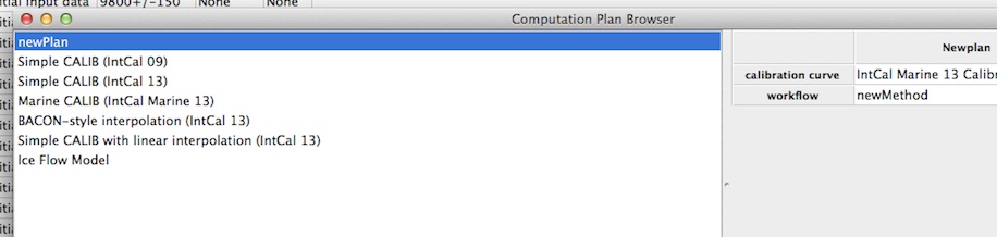
If you want to see what steps are involved in a particular scientific workflow, you use the Computation Plan Browser, which you can find by clicking "Tools" at the very top left of your screen, then using the dropdown to select "Computation Plan Browser." You'll get a screen like this:
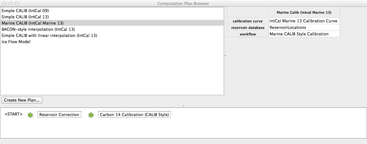 |
If you click on one of the workflow names in the upper left hand box of the Computation Plan Browser window, you'll see what steps are involved in that workflow. In the image above, I've clicked on "Marine CALIB (IntCal Marine 13)", as you can tell because it's highlighted in grey. That workflow has two steps, shown schematically in the bottom half of that window: a reservoir age correction and a CALIB-style 14C calibration.
CSciBox has a number of built-in "computation plan elements" -- chunks of code that perform standard, useful steps in paleodata analysis. Many of these computational elements involve supporting data sets, such as 14C calibration curves. The operative ones for a given workflow appear in the top right part of the Computation Plan Browser window when you're looking at that workflow. In the screenshot just above, there are two: ReservoirLocations, a table of reservoir age corrections that we downloaded from the 14CHRONO website and stored in CSciBox's database, and the IntCal Marine 13 calibration curve, which was downloaded from Radiocarbon.
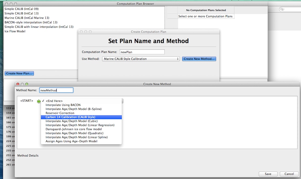
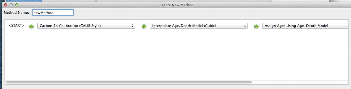
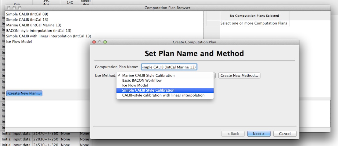
You can also make a new analysis workflow using the Computation Plan Browser by clicking on the "Create New Plan" button (just above the "Start" icon in the screenshot above) and typing a name into the "Computation Plan Name" box. CSciBox has a bunch of templates -- called "Methods," for lack of a better name -- that allow you to easily build new variants on existing computation plans that use different background data sets: that is, the blocks in the plan are exactly the same, but the data sets that they us (e.g., which IntCal curve, which reservoir age data set) are different. Here are some of those templates:
 |
 |
 |
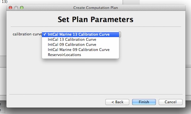
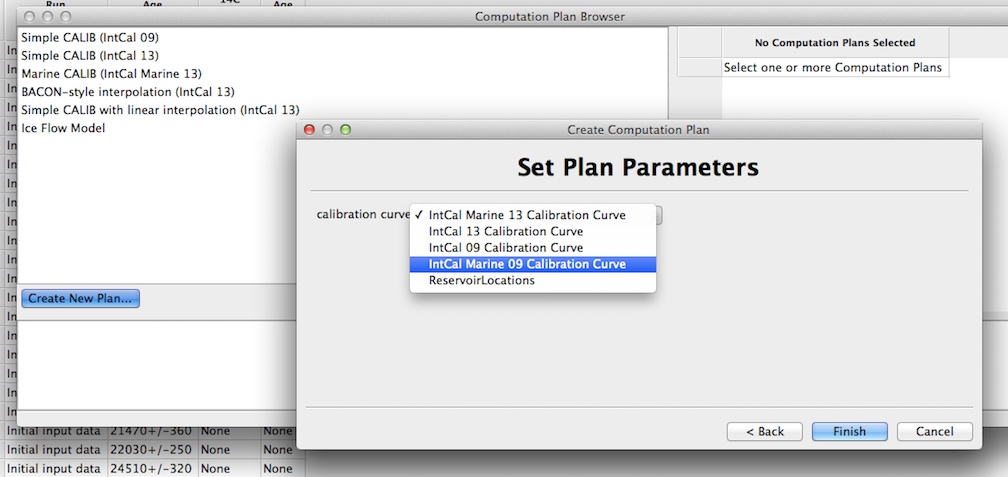
Next you click 'save.' If your new plan requires a choice regarding a calibration or other background data set, CSciBox will ask you about that choice. Here, since I've included a CALIB-style Carbon 14 calibration step, CSciBox needs to know what calibration curve to use:
 |
After clicking on 'finish' and 'next', that new plan will appear in the main computation-plan browser window (top left, below):
 |
If you had just wanted to make a minor modification on an existing workflow -- say, using a different calibration curve in the CALIB step of the plan in the example above -- you wouldn't need to create a new method. (You only create a new method when you want to actually put together a computation plan that has a different set of computational blocks than any existing one.) Rather, you'd select one of the existing methods:
 |
 |
 |